COMSOL 不确定性量化模块——理解和表征模型的不确定性_公司动态

输入参数和关注量

在运行不确定性量化研究时，您可以根据 COMSOL Multiphysics® 模型的解来定义一组关注量。这样一来，关注量就成了输入参数的函数。

在结构分析的情况下，关注量可以是最大位移、应力或偏转角。对于传热或 CFD 分析，关注量可以是最高温度、总热损耗或总流体流率。对于电磁仿真，则可以是电阻、电容或电感。由于“不确定性量化模块”适用于使用 COMSOL Multiphysics® 软件计算的任何物理场模型，以及各种求解场量的数学表达式，因此关注量的选择是无穷无尽的。

任何不确定的模型输入，无论是物理场设置、几何尺寸、材料属性还是离散化设置，都可以作为输入参数，并且任何模型输出都可以用来定义关注量。

筛选

筛选，MOAT 研究类型实现了一种轻量级的全局筛选方法，可以对每个输入参数的重要性进行定性度量。该方法纯粹基于样本，使用 Morris one-at-a-time（MOAT）方法，所需的 COMSOL 模型计算量相对较小。当输入参数的数量太大而无法进行计算成本较高的不确定性量化研究时，这使其成为一种理想的方法。

对于每个关注量，MOAT 方法计算每个输入参数的 MOAT 平均值和标准差，并将它们显示在 MOAT 散点图中。MOAT 平均值和标准差的排序给出了输入参数的相对重要性。前者越高意味着该参数显著影响关注量，后者越高则意味着该参数会产生影响，并且它要么与其他参数有很强的相互作用，要么具有非线性影响，或两者兼而有之。

COMSOL Multiphysics 用户界面，显示了“模型开发器”，其中突出显示“不确定性量化”节点，并显示其对应的“设置”窗口；“图形”窗口中显示 MOAT 散点图。

关注量的 Sobol 指数图，其中 x1 显示为蓝色条，x2 为绿色条，x3 为红色条，x4 为青色条。

灵敏度分析

灵敏度分析 研究类型用于计算关注量对输入参数的敏感性，包含两种方法：Sobol 法和相关法。

Sobol 法用于分析整个输入参数分布，并将每个关注量的方差分解为输入参数及其相互作用的贡献之和。

Sobol 法可以计算每个输入参数的 Sobol 指数。一阶 Sobol 指数显示由各个输入参数的方差产生的关注量的方差。总 Sobol 指数显示由每个输入参数的方差及其与其他输入参数的相互作用而产生的关注量的方差。每个关注量和所有参数的 Sobol 指数都显示在专用的 Sobol 图中，其中直方图按总 Sobol 指数排序。关注量对具有最高总 Sobol 指数的输入参数最敏感。输入参数的总 Sobol 指数和一阶 Sobol 指数之间的差异可以衡量该输入与其他输入之间相互作用的效果。

与筛选方法相比，灵敏度分析用于定量分析关注量的不确定性如何分配给不同的输入参数。这种方法需要更多的计算资源，原因是精确的 Sobol 指数计算依赖于高质量的代理模型。

相关法可以计算每个输入参数与关注量之间的线性和单调关系。对于基于相关法的灵敏度分析，可以计算四种类型的相关性：双变量相关、等级双变量相关、偏相关或等级偏相关。

不确定性传播

不确定性传播 研究类型用于分析输入参数的不确定性如何通过计算其概率密度函数（PDF）传播到每个关注量。大多数通过 COMSOL Multiphysics® 模型计算来将输入参数与关注量进行映射的底层物理应用通常是无法进行解析计算的。

因此，需要进行蒙特卡罗分析来近似得到 PDF。与 Sobol 法类似，使用代理模型可以显著降低蒙特卡罗分析的计算成本。对于每个关注量，都可以执行核密度估计（KDE），并为其生成可视化效果图，作为 PDF 的近似值。此外，置信区间表可以基于此分析给出每个关注量的平均值、标准差、最小值、最大值以及对应于 90%、95% 和 99% 置信水平的下限值和上限值。

可靠性分析

与用于探索关注量的总体不确定性的其他不确定性量化研究类型相比，可靠性分析，EGRA 方法可以解决更直接的问题。给定一个标称设计和一些特定的不确定输入，设计失败的概率是多少？失败的原因可以是设计的完全失效，也可以用质量准则来表述。

为了确保可靠性，传统的建模仿真方法是使用安全裕度和最坏情况。通过适当的可靠性分析，可以计算实际概率，从而避免高估和低估结果。从每个关注量的不确定性传播的置信区间表中可以得到粗略估计。但是通过可靠性分析，您可以根据关注量和相应阈值的组合来定义更复杂的可靠性准则。用于可靠性分析研究的高效全局可靠性分析（EGRA）方法可以有效地将计算资源引导至区分设计失败和成功的极限状态。

代理模型和响应面

使用 Sobol 法计算的灵敏度分析、不确定性传播和可靠性分析都依赖于精确的蒙特卡罗型分析，这通常需要大量的计算才能达到良好的准确性。对于 COMSOL Multiphysics® 模型计算可能需要大量资源且不确定性量化分析涉及多个参数的现实问题，仅使用 COMSOL Multiphysics® 模型计算进行的蒙特卡罗分析在计算上并不可行。“不确定性量化模块”的一个关键特点是，它能够针对特定的 UQ 分析训练和使用代理模型（也称为元模型），从而节省计算资源。

代理模型是一种紧凑的数学模型，用于表示和计算由输入参数定义的关注域中的关注量。这种模型完全独立于基础 COMSOL Multiphysics® 模型，并且在经过适当的训练后，可用于代替 COMSOL Multiphysics® 模型来预测其他输入参数值的关注量的值，而不是求解的值。构造代理模型的过程通常是自适应的，并且代理模型可以高精度地近似原始模型。用户定义的容差可以提高代理模型的准确性。更高级别的准确性需要额外的 COMSOL Multiphysics® 模型计算。

一旦建立代理模型，您就可以进行独立验证以进一步测试其有效性，并可以快速计算整个输入参数空间的响应面数据。然后，可以将响应面进行可视化，其中每次绘制一个关注量与两个输入参数的关系。

Six plots displayed in a stacking sequence, with three plots in the Rainbow color table.

Inverse Uncertainty Quantification

Inverse uncertainty quantification (inverse UQ) is used when some of the input parameters have unknown probability distributions, known as calibration parameters. Using inverse UQ, experimental data can be propagated backward to gain insight into the statistical properties of these calibration parameters. In order to apply inverse UQ, a prior probability distribution is required for each calibration parameter before the analysis can be conducted.

Experimental data is typically available for the quantities of interest and the parameters used in experiments. There are also calibration input parameters that cannot be directly measured. For instance, consider an experiment where we want to calibrate the Young's modulus of a mechanical part. We should conduct an experiment that measures the tensile stress as a function of the specified material displacement. An inverse UQ study should then be set up to use the experimental data and prior knowledge of the Young's modulus to calibrate the probability distribution that would best reproduce the measured values of the tensile stress from the experiments. Inverse UQ can be applied to a wide range of physics-based models, including those related to structural mechanics, fluid flow, acoustics, heat transfer, electromagnetics, and chemical engineering.

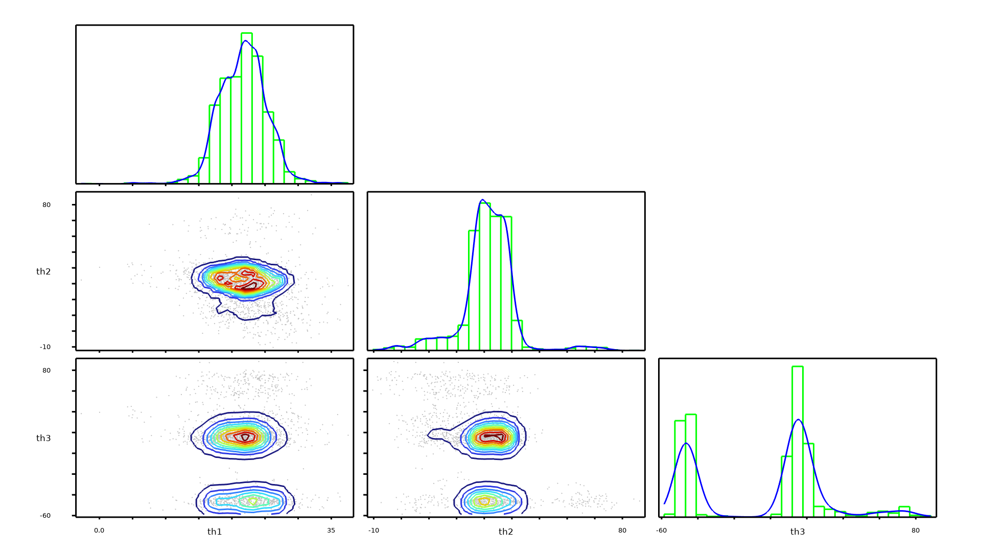
To make the computation of the calibration parameters' posterior probability distributions feasible, a surrogate model is used together with a Markov chain Monte Carlo (MCMC) method. After the computation, the joint and marginal probability distributions of the calibrated input parameters can be visualized. Additionally, a confidence interval table is generated that provides information such as the mean; the standard deviation; the minimum and maximum values; and the lower- and upper-bound values corresponding to confidence levels of 90%, 95%, and 99% for each calibrated input parameter.

公司动态